Python for Geospatial Data Analysis

CoPhil EO AI/ML Training - Day 1, Session 3

Stylianos Kotsopoulos

EU-Philippines CoPhil Programme

Welcome to Session 3

Session Overview

Python for Geospatial Data Analysis

Hands-on introduction to working with vector and raster data using Python

Format: Brief conceptual intro + Extended hands-on coding

Duration: 2 hours (15-20 min presentation + 100 min hands-on)

Learning Objectives

By the end of this session, you will be able to:

1. Set up and use Google Colaboratory for geospatial analysis
2. Load, explore, and visualize vector data with GeoPandas
3. Read, process, and visualize raster data with Rasterio
4. Perform basic geospatial operations (clipping, reprojecting, cropping)
5. Prepare data for AI/ML workflows

Session Roadmap

Time	Topic	Duration
00-15 min	Setup & Python Basics Recap	15 min
15-55 min	GeoPandas for Vector Data (HANDS-ON)	40 min
55-60 min	☕ Break	5 min
60-110 min	Rasterio for Raster Data (HANDS-ON)	50 min
110-120 min	Summary & Next Steps	10 min

Timing: 2 minutes

Key Point: This is a HANDS-ON session. Participants code along in their notebooks.

Notebook Access

📓 Google Colab Notebook:

Day1_Session3_Python_Geospatial_Data.ipynb

1. Open link from course materials
2. Save a copy to your Drive
3. Run first cell to install packages
4. Follow along as we code together

Timing: 3 minutes

Instructor Actions: - Share notebook link in chat - Wait for participants to open and save copy - Verify everyone can see the notebook - Explain Colab basics (cells, shift+enter)

Troubleshooting: - “Can’t access?” → Check Google account login - “Packages fail?” → Restart runtime

Today’s Focus

Vector Data:

• Administrative boundaries
• Points of interest
• Roads, rivers
• Training sample polygons
• Using GeoPandas

Raster Data:

• Satellite imagery
• Digital elevation models
• Land cover maps
• AI model outputs
• Using Rasterio

Integration: Combining vector and raster for complete EO workflows

Why Python for Geospatial?

The Python Advantage

Why Python is the Leading Language for EO:

1. Rich Ecosystem
   • Hundreds of specialized libraries
   • Active development and community
2. Easy to Learn
   • Clear syntax, readable code
   • Gentle learning curve
3. Powerful Integration
   • Connects data sources, processing, ML
   • Single environment for complete workflows
4. Free and Open Source
   • No licensing costs
   • Transparent and reproducible

Python Geospatial Ecosystem

Complete Python Earth Observation Ecosystem organized by function

This diagram shows the complete Python ecosystem for Earth Observation, organized by function: Data Access (Earth Engine, Sentinel Hub), Geospatial Processing (GeoPandas, Rasterio), Data Science (NumPy, Pandas), Machine Learning (Scikit-learn, TensorFlow, PyTorch), and Visualization tools. Notice how data flows from access through processing to analysis and visualization.

Integration Capabilities

Python Connects Everything:

# Example workflow
import geopandas as gpd
import rasterio
from sklearn.ensemble import RandomForestClassifier

# Load vector training data
training = gpd.read_file('samples.geojson')

# Load satellite raster
with rasterio.open('sentinel2.tif') as src:
    image = src.read()

# Extract features and train model
X, y = extract_features(image, training)
model = RandomForestClassifier()
model.fit(X, y)

# Predict on full image
prediction = model.predict(image)

Community and Resources

Vibrant Python Geospatial Community:

Documentation:

• Comprehensive guides for all libraries
• Tutorials and examples
• API references

Community Support:

• Stack Overflow
• GitHub discussions
• GIS Stack Exchange
• Dedicated forums

Learning Resources:

• Free courses (Coursera, Udemy)
• Books (Automating GIS Processes)
• Blogs and tutorials
• Conference workshops

Google Colaboratory

Why Colab for This Training?

Advantages for Learning:

1. No Setup Hassles
   • Works immediately
   • No environment configuration
   • Consistent for all participants
2. Accessible Anywhere
   • Just need a browser
   • Works on any computer
   • Even tablets
3. Powerful Resources
   • Free GPU for deep learning
   • 12+ GB RAM
   • Sufficient for all exercises
4. Easy Sharing
   • Share notebooks instantly
   • Collaborative editing
   • CoPhil materials readily accessible

Colab Interface Overview

Main Components:

1. Menu Bar
   • File, Edit, View, Insert, Runtime

2. Toolbar
   • Play button to run cells
   • Add code/text cells

3. Notebook Area
   • Code cells (executable)
   • Text cells (Markdown)

4. Sidebar
   • Table of contents
   • Files browser
   • Code snippets

Colab Interface

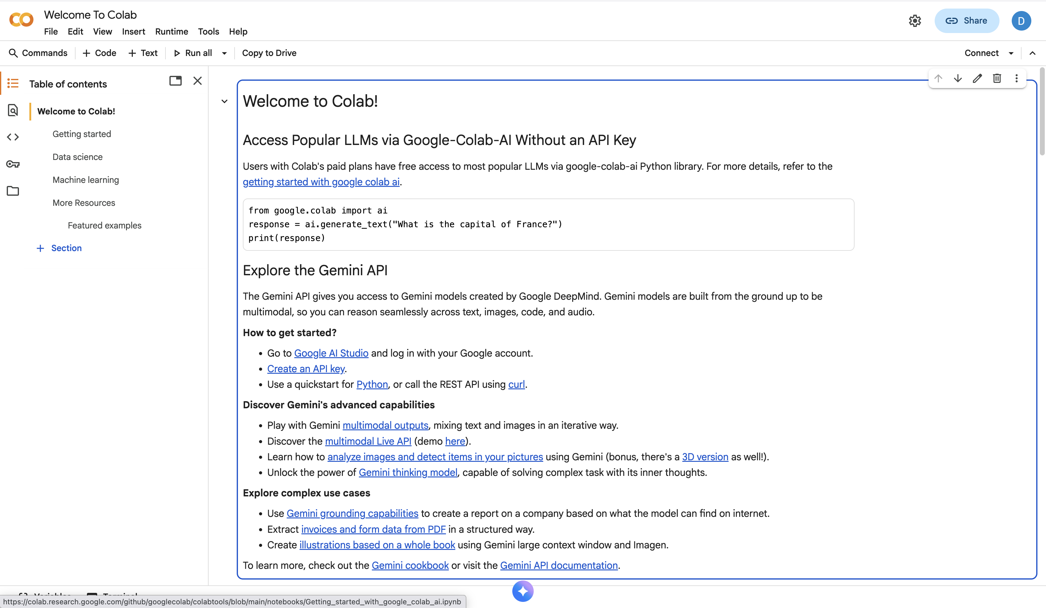
Running Code in Colab

Two Ways to Execute Cells:

1. Click the Play Button

• Left side of each code cell
• Runs that specific cell

2. Keyboard Shortcuts

• Shift + Enter: Run cell and move to next
• Ctrl + Enter: Run cell, stay on current
• Ctrl + M then A: Add cell above
• Ctrl + M then B: Add cell below

Output Appears Below Cell:

Text, plots, tables, errors all display inline.

Google Drive Integration

Mounting Your Google Drive:

from google.colab import drive
drive.mount('/content/drive')

Benefits:

• Persistent storage (Colab resets)
• Upload/download data
• Save outputs
• Share files between notebooks

Access Your Files:

# Your Drive files appear at:
# /content/drive/MyDrive/

# Example:
import geopandas as gpd
gdf = gpd.read_file('/content/drive/MyDrive/data/boundaries.shp')

Installing Additional Packages

Most Common Libraries Pre-Installed:

NumPy, Pandas, Matplotlib, Scikit-learn

For Geospatial Libraries:

# GeoPandas (usually pre-installed, but check version)
!pip install geopandas

# Rasterio
!pip install rasterio

# Other useful libraries
!pip install earthengine-api
!pip install folium

Note: Packages need reinstalling each session (Colab resets runtime)

GeoPandas for Vector Data

What is GeoPandas?

Pandas + Geometry = GeoPandas

Definition:

Extension of Pandas for working with geospatial vector data

Key Concept:

Like a spreadsheet/table where one column contains geometries (points, lines, polygons)

Built On:

• Pandas - Data manipulation
• Shapely - Geometric operations
• Fiona - File I/O
• PyProj - Coordinate systems

GeoPandas

Pandas + Geometry

The GeoDataFrame Concept

Similar to Pandas DataFrame:

Regular DataFrame:

Name	Population	Area
Manila	1.78M	42.88
Cebu	0.92M	315
Davao	1.63M	2444

GeoDataFrame:

Name	Population	Area	geometry
Manila	1.78M	42.88	POLYGON(…)
Cebu	0.92M	315	POLYGON(…)
Davao	1.63M	2444	POLYGON(…)

Special “geometry” Column:

Contains spatial information (coordinates defining shapes)

Common Vector Data Operations

What You Can Do with GeoPandas:

1. Read/Write
   • Shapefiles, GeoJSON, GeoPackage, PostGIS
2. Explore
   • View attributes, examine geometries
3. Visualize
   • Quick plotting, interactive maps
4. Geoprocessing
   • Buffer, intersection, union, clip
5. Spatial Joins
   • Combine datasets based on location
6. Coordinate Transformations
   • Reproject to different CRS

GeoPandas Code Example

Loading and Visualizing:

import geopandas as gpd
import matplotlib.pyplot as plt

# Read Philippine provinces shapefile
provinces = gpd.read_file('philippines_provinces.shp')

# Examine data
print(provinces.head())
print(provinces.crs)  # Check coordinate system

# Simple plot
provinces.plot(figsize=(10, 10),
               edgecolor='black',
               facecolor='lightblue')
plt.title('Philippine Provinces')
plt.show()

Visualization Capabilities

GeoPandas Plotting:

# Color by attribute
provinces.plot(column='population',
               cmap='YlOrRd',
               legend=True,
               figsize=(12, 10))
plt.title('Population by Province')

# Add basemap (with contextily)
import contextily as ctx
provinces_web_mercator = provinces.to_crs(epsg=3857)
ax = provinces_web_mercator.plot(figsize=(15, 15),
                                   alpha=0.5)
ctx.add_basemap(ax)

GeoPandas integrates seamlessly with Matplotlib for static plots and can work with Folium or Plotly for interactive maps. For training, we’ll focus on quick visualization for QA and exploration.

Philippine Coordinate Reference Systems

Common CRS for Philippines:

EPSG	Name	Type	Units	Use Case
4326	WGS84	Geographic	Degrees	Web maps, lat/lon
32651	UTM Zone 51N	Projected	Meters	Western PH, Manila
32652	UTM Zone 52N	Projected	Meters	Eastern PH, Mindanao
3123	PRS92 Zone III	Projected	Meters	National standard

Rule: Use geographic (4326) for storage, projected (UTM) for analysis

Philippines spans two UTM zones. Zone 51N covers Manila, Palawan, western areas. Zone 52N covers Mindanao and eastern regions. Always reproject to UTM for area/distance calculations!

Philippine UTM Zones

UTM Zone 51N (EPSG:32651)

Coverage: - Metro Manila - Palawan - Western Luzon - Western Visayas

Most common for: - Urban analysis - Palawan studies - Manila projects

UTM Zone 52N (EPSG:32652)

Coverage: - Mindanao - Eastern Visayas - Bicol Region - Eastern Luzon

Most common for: - Mindanao analysis - Disaster mapping - Agricultural studies

Code Example:

# Reproject to UTM 51N for area calculation
gdf_utm = gdf.to_crs(epsg=32651)
gdf_utm['area_km2'] = gdf_utm.geometry.area / 1_000_000

The UTM zone boundary runs roughly through the middle of the Philippines. For national-scale work, pick one zone and reproject everything to it, or use PRS92.

Philippine Geospatial Data Sources

NAMRIA Geoportal - Administrative boundaries - Topographic maps - Land cover 2020 - DEMs - www.geoportal.gov.ph

PhilSA - Satellite imagery - EO products - philsa.gov.ph

PSA - Census boundaries - Barangay data - psa.gov.ph

OpenStreetMap - Roads, buildings - extract.bbbike.org

Natural Earth - Country boundaries - naturalearthdata.com

All work with GeoPandas - just gpd.read_file()!

NAMRIA is the official source for government work. OSM is community-maintained but very detailed for urban areas. PhilSA provides satellite-derived products.

Rasterio for Raster Data

What is Rasterio?

Python Wrapper for GDAL

Definition:

Clean, idiomatic Python library for reading and writing geospatial raster data

Why Not Use GDAL Directly?

• GDAL Python bindings are cumbersome
• Rasterio is more Pythonic
• Better integration with NumPy
• Cleaner syntax

Works With:

All formats GDAL supports - GeoTIFF, COG, NetCDF, HDF, etc.

Rasterio

Python Wrapper for GDAL

Raster Data Structure

How Rasterio Represents Imagery:

3D NumPy Array:

(bands, rows, columns)

Example: Sentinel-2 10m Bands:

# 4 bands (Blue, Green, Red, NIR)
# 1098 rows (10980 m / 10 m)
# 1098 columns (10980 m / 10 m)
# Shape: (4, 1098, 1098)

array[0, :, :]  # Band 1 (Blue)
array[1, :, :]  # Band 2 (Green)
array[2, :, :]  # Band 3 (Red)
array[3, :, :]  # Band 4 (NIR)

Reading Raster Data with Rasterio

Basic Workflow:

import rasterio
import numpy as np

# Open raster file
with rasterio.open('sentinel2_10m.tif') as src:
    # Read all bands
    data = src.read()

    # Read specific band
    red_band = src.read(3)

    # Get metadata
    print(f"CRS: {src.crs}")
    print(f"Transform: {src.transform}")
    print(f"Width: {src.width}, Height: {src.height}")
    print(f"Bounds: {src.bounds}")
    print(f"Number of bands: {src.count}")

The ‘with’ statement ensures the file is properly closed after reading. This is good practice and prevents file locking issues.

Array Operations

Rasterio + NumPy = Powerful Processing

# Calculate NDVI
with rasterio.open('sentinel2_10m.tif') as src:
    red = src.read(3).astype(float)
    nir = src.read(4).astype(float)

# NDVI formula
ndvi = (nir - red) / (nir + red + 1e-8)  # Small value prevents division by zero

# Apply threshold
vegetation_mask = ndvi > 0.3

# Calculate statistics
print(f"Mean NDVI: {np.mean(ndvi):.3f}")
print(f"Vegetation pixels: {np.sum(vegetation_mask)}")

Common Spectral Indices

Key Indices for EO Analysis:

Index	Formula	Purpose	Range
NDVI	(NIR - Red) / (NIR + Red)	Vegetation health	-1 to +1
EVI	2.5 × (NIR - Red) / (NIR + 6×Red - 7.5×Blue + 1)	Enhanced vegetation	-1 to +1
NDWI	(Green - NIR) / (Green + NIR)	Water bodies	-1 to +1
NDBI	(SWIR - NIR) / (SWIR + NIR)	Built-up areas	-1 to +1

Sentinel-2 Bands: Blue (B2), Green (B3), Red (B4), NIR (B8), SWIR (B11, B12)

These indices are fundamental for EO analysis. NDVI is most common for vegetation. EVI better in high biomass areas (tropical forests). NDWI for flood mapping.

Philippine Application: Rice Monitoring

Using NDVI for Philippine Rice Paddies:

# Calculate NDVI for Central Luzon rice area
with rasterio.open('sentinel2_central_luzon.tif') as src:
    red = src.read(4).astype(float)   # Band 4
    nir = src.read(8).astype(float)   # Band 8

# NDVI calculation
ndvi = (nir - red) / (nir + red + 1e-8)

# Classify vegetation health
bare_soil = ndvi < 0.2      # Recently planted / fallow
growing = (ndvi >= 0.2) & (ndvi < 0.5)  # Early growth
mature = (ndvi >= 0.5) & (ndvi < 0.8)   # Peak biomass
very_dense = ndvi >= 0.8    # Maximum vegetation

# Calculate rice area statistics
pixel_area = 100  # 10m x 10m = 100 m²
mature_rice_area_ha = np.sum(mature) * pixel_area / 10000

print(f"Mature rice area: {mature_rice_area_ha:.2f} hectares")

This workflow is used by PRiSM for operational rice monitoring across the Philippines. NDVI time series tracks crop phenology from planting to harvest.

Visualization with Rasterio

Displaying Satellite Imagery:

import matplotlib.pyplot as plt
from rasterio.plot import show

# Open and display
with rasterio.open('sentinel2_10m.tif') as src:
    # Show true color composite (RGB)
    show((src, [3, 2, 1]), title='True Color')

    # Show false color composite (NIR, Red, Green)
    show((src, [4, 3, 2]), title='False Color (NIR-R-G)')

# Or read and plot with matplotlib
with rasterio.open('sentinel2_10m.tif') as src:
    data = src.read([3, 2, 1])  # RGB
    # Scale to 0-255 for display
    data_scaled = np.clip(data / 3000, 0, 1)

    plt.figure(figsize=(10, 10))
    plt.imshow(np.moveaxis(data_scaled, 0, -1))
    plt.title('Sentinel-2 True Color')
    plt.axis('off')
    plt.show()

Hands-On Preview

What We’ll Build Today

Notebook 1: Vector Data with GeoPandas

1. Load Philippine administrative boundaries
2. Explore and visualize provinces
3. Filter specific regions (e.g., Central Luzon)
4. Calculate area and basic statistics
5. Spatial operations (buffer, clip)
6. Create training sample polygons

What We’ll Build Today

Notebook 2: Raster Data with Rasterio

1. Load Sentinel-2 image subset
2. Examine metadata and properties
3. Visualize true and false color composites
4. Calculate vegetation indices (NDVI, EVI)
5. Crop to area of interest
6. Extract pixel values at point locations
7. Save processed outputs

Integrating Vector and Raster

Combining Both Data Types:

import geopandas as gpd
import rasterio
from rasterio.mask import mask

# Load vector boundary
aoi = gpd.read_file('study_area.geojson')

# Load raster
with rasterio.open('sentinel2.tif') as src:
    # Clip raster to vector boundary
    clipped_data, clipped_transform = mask(
        src,
        aoi.geometry,
        crop=True
    )

    # Update metadata for output
    out_meta = src.meta.copy()
    out_meta.update({
        "height": clipped_data.shape[1],
        "width": clipped_data.shape[2],
        "transform": clipped_transform
    })

Preparing for ML Workflows

What You’ll Learn:

1. Extract Training Data
   • Sample raster values at polygon locations
   • Create feature matrix (X) and labels (y)
2. Spatial Data Splits
   • Avoid spatial autocorrelation in train/test
3. Data Formatting
   • Structure for Scikit-learn, TensorFlow, PyTorch
4. Quality Control
   • Check for NaN values, outliers
   • Validate spatial alignment

Link to Colab Notebooks

Access Today’s Notebooks:

Notebook 1: Vector Data

[Link will be provided in chat]

Notebook 2: Raster Data

[Link will be provided in chat]

Make a Copy:

File → Save a copy in Drive (so you can edit and experiment)

Tips for Success

As We Work Through Notebooks:

1. Run Cells Sequentially
   • Top to bottom order matters
   • Each cell may depend on previous
2. Read the Comments
   • Explanations included in code
   • Learn the “why” not just “how”
3. Experiment
   • Modify parameters
   • Try different visualizations
   • Break things and learn
4. Ask Questions
   • Use chat or raise hand
   • No question is too basic
5. Take Notes
   • Useful patterns and code snippets
   • Errors and solutions

Key Concepts Summary

Python Geospatial Ecosystem

GeoPandas:

• DataFrame + geometry column
• Vector data operations
• Easy visualization
• Integration with Pandas

Rasterio:

• Clean GDAL wrapper
• NumPy array representation
• Comprehensive metadata handling
• Efficient I/O

Integration:

• Both work together seamlessly
• Complete EO workflows in Python
• Foundation for ML/AI applications

Why These Skills Matter

For AI/ML in Earth Observation:

1. Data Preparation
   • Loading and preprocessing is 80% of work
   • Quality in → Quality out
2. Feature Engineering
   • Calculate indices, textures, derivatives
   • NumPy operations on raster arrays
3. Training Data Creation
   • Sample raster at polygon locations
   • Extract features for supervised learning
4. Model Deployment
   • Apply trained models to new imagery
   • Generate prediction maps
5. Validation and QA
   • Compare predictions to ground truth
   • Calculate accuracy metrics

Building Blocks for This Week

Today’s Skills Enable:

Day 2:

• Random Forest land cover classification
• Preparing training data for ML

Day 3:

• Deep learning data pipelines
• U-Net flood mapping inputs

Day 4:

• Time series data preparation
• LSTM input formatting

Mastering these fundamentals now will make everything else smoother.

☕ 5-Minute Break

Stretch Break

Stand up • Grab water • Back in 5 minutes

Timing: 5 minutes

After Break: Continue with Rasterio section (50 minutes of hands-on coding)

Let’s Begin!

Transition to Hands-On

Open Your Notebooks

We’ll start with:

Vector Data Analysis using GeoPandas

Remember:

• Make a copy of the notebook
• Mount your Google Drive
• Run cells in order
• Ask questions anytime

Support During Hands-On

Instructors Available:

• Main instructor demonstrating
• Teaching assistants in chat
• Screen sharing for debugging

Pacing:

• We’ll work through together
• Pause points for questions
• Extra exercises for fast finishers

Goal:

Everyone completes core exercises, understands concepts, ready for GEE

Session Complete!

Session Summary

What You’ve Learned:

✅ Google Colab setup for geospatial work
✅ GeoPandas for vector data (load, visualize, analyze)
✅ Rasterio for raster data (read, process, visualize)
✅ Coordinate systems and projections
✅ Basic geospatial operations (clip, reproject, crop)
✅ Data preparation for ML workflows

Timing: 3 minutes

You now have foundational Python geospatial skills. Session 4 builds on this with Google Earth Engine.

Q&A

Common Questions:

• GeoPandas vs Shapely?
• When to use Rasterio vs GDAL?
• CRS issues and solutions?
• Memory errors with large files?

• Best practices for file paths?
• NoData values handling?
• Visualization tips?
• Integration with ML pipelines?

Common Answers: - GeoPandas uses Shapely under the hood - Rasterio = Pythonic GDAL wrapper - Always check CRS before operations - Use chunking/windowing for large rasters

Next: Session 4

Google Earth Engine

Coming up:

• Cloud-based EO data processing
• Access to entire Sentinel archive
• Planetary-scale analysis
• Python API (geemap)
• Cloud masking & compositing
• Export workflows

Get ready for GEE! 🌍

Everyone completes core exercises with understanding, not just copying code.

Questions Before We Start?

Any questions about the tools or approach?

Take a few questions, then transition to the hands-on Colab notebooks. The rest of the session will be interactive coding with support.

Let’s Code!

Opening Notebook 1: GeoPandas for Vector Data