Introduction to Google Earth Engine

CoPhil EO AI/ML Training - Day 1, Session 4

Stylianos Kotsopoulos

EU-Philippines CoPhil Programme

Welcome to Session 4

Final Session of Day 1!

Google Earth Engine

Planetary-scale geospatial analysis in the cloud

Duration: 2 hours (Hands-on with Python API)

This session introduces Google Earth Engine using Python exclusively (no JavaScript Code Editor). Participants will use geemap library for Python-based GEE access.

Learning Objectives

By the end of this session, you will be able to:

1. Understand what GEE is and why it’s powerful
2. Authenticate and initialize GEE Python API
3. Access Sentinel-1 and Sentinel-2 imagery
4. Filter image collections (spatial, temporal, property)
5. Apply cloud masking to Sentinel-2
6. Create temporal composites (median, mean)
7. Calculate spectral indices (NDVI, NDWI)
8. Visualize results with geemap
9. Export data for further analysis

Session Roadmap

Time	Topic	Duration
00-15 min	GEE Overview & Authentication	15 min
15-55 min	Core Concepts & Sentinel Access (HANDS-ON)	40 min
55-60 min	☕ Break	5 min
60-110 min	Processing & Visualization (HANDS-ON)	50 min
110-120 min	Export & Summary	10 min

Timing: 2 minutes

Like Session 3, this is heavily hands-on. Most time spent coding in notebooks following instructor demonstration.

Part 1: Google Earth Engine Overview

What is Google Earth Engine?

Cloud-Based Platform for Geospatial Analysis

• Massive data catalog (petabytes)
• Powerful compute (Google’s infrastructure)
• Free for research & education
• No download needed
• Process at scale

“Planetary-scale geospatial analysis”

Timing: 3 minutes

Key Points: - GEE hosts 40+ years of satellite imagery - Entire Landsat, Sentinel, MODIS archives - Processing happens on Google’s servers, not your laptop - Analyze entire countries in minutes - Free tier sufficient for most research/education

GEE Architecture and Workflow

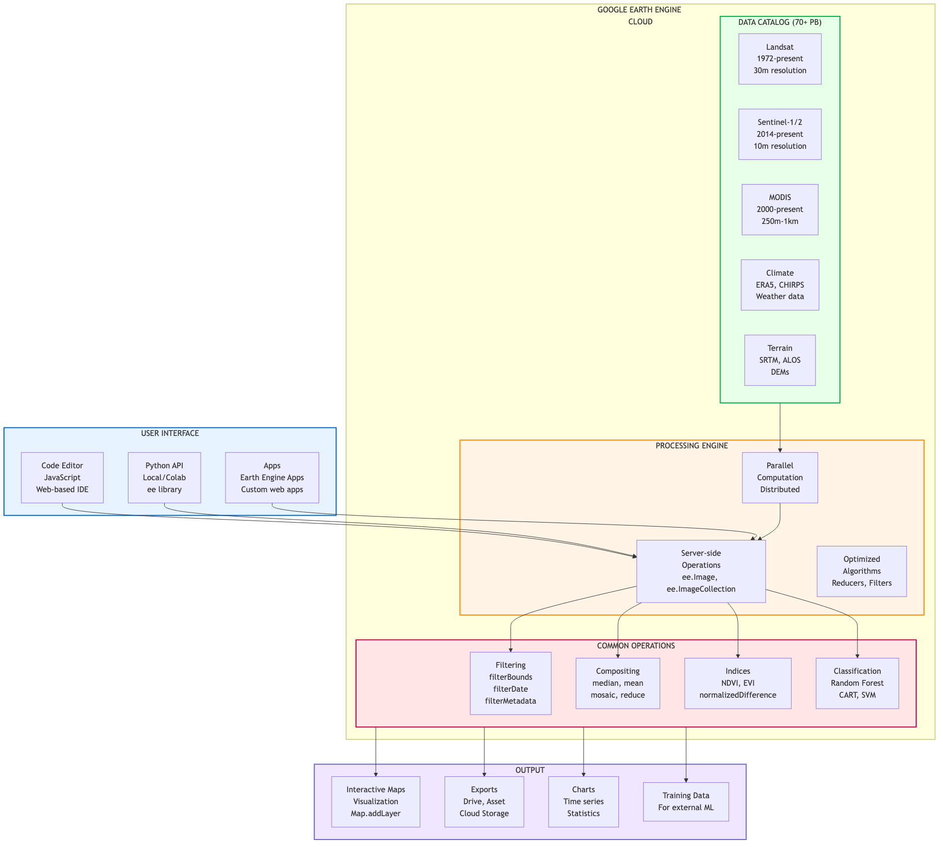
Google Earth Engine complete architecture showing User Interface, Cloud Processing, Data Catalog, and Outputs

This comprehensive diagram shows GEE’s architecture: multiple user interfaces (Code Editor, Python API, Apps), the massive data catalog (70+ PB including Landsat, Sentinel, MODIS), distributed processing engine, common operations (filtering, compositing, indices, classification), and various output options (maps, exports, charts, training data).

Why GEE for This Training?

Addresses Key Challenges:

• ❌ Traditional: Download 100s of GB of Sentinel data

• ✅ GEE: Access entire archive without downloading

• ❌ Traditional: Need powerful computer for processing

• ✅ GEE: Google’s infrastructure does the work

• ❌ Traditional: Complex cloud masking & preprocessing

• ✅ GEE: Built-in algorithms & analysis-ready data

• ❌ Traditional: Time-series analysis is painful

• ✅ GEE: Designed for temporal analysis

Perfect for Philippine-scale analysis!

GEE Data Catalog

Datasets Available:

Satellite Imagery:

• Sentinel-1, 2, 3, 5P
• Landsat (entire archive!)
• MODIS
• Planet, SkySat (some)
• Many more…

Geophysical:

• Climate data
• Elevation (SRTM, ASTER)
• Weather data
• Population datasets
• Land cover products

Browse: https://developers.google.com/earth-engine/datasets

GEE hosts 800+ public datasets. All preprocessed and analysis-ready. Focus today on Sentinel-1 and Sentinel-2.

Python API vs JavaScript Code Editor

JavaScript Code Editor

• Web-based IDE
• Interactive visualization
• Quick prototyping
• Built-in examples

Python API (Our Focus)

• Jupyter notebooks
• Integration with ML libraries
• Familiar Python ecosystem
• geemap package for visualization

Today: Python-only approach using geemap

Why Python for this training: - Integrates with ML workflows (scikit-learn, TensorFlow, PyTorch) - Familiar to data scientists - geemap provides all visualization capabilities - Better for reproducible research

geemap Package

Python package for interactive GEE mapping

• Built on ipyleaflet
• Interactive map visualization
• Layer controls
• Inspector tool
• Split-panel comparison
• Export functionality
• Makes Python GEE as easy as Code Editor

geemap by Dr. Qiusheng Wu. Makes GEE accessible from Jupyter. We’ll use it extensively today.

GEE Authentication

Sign Up for GEE

Before We Code

You need a Google Earth Engine account!

Sign up: https://earthengine.google.com/signup

Steps:

1. Visit signup page
2. Use Gmail account
3. Select “Research/Education”
4. Wait for approval (usually instant)

Already have account? Great! Let’s authenticate.

Timing: 2 minutes

Check: Ask participants if everyone has GEE access approved. If not, they can follow along and authenticate later.

Authentication Process

83d Open Notebook: Day1_Session4_Google_Earth_Engine.ipynb

Authentication Code:

import ee
import geemap

# Authenticate (first time only)
ee.Authenticate()

# Initialize
ee.Initialize()

print("GEE Initialized Successfully!")

Timing: 5 minutes - participants authenticate

Steps: 1. Run ee.Authenticate() - opens browser tab 2. Sign in with Google account 3. Allow Earth Engine access 4. Copy token back to notebook 5. Run ee.Initialize() 6. Confirm success message

Troubleshooting: - “Authentication failed” → Check GEE account approved - “Module not found” → Install geemap: pip install geemap

Part 2: Core GEE Concepts

Key GEE Objects

ee.Image

• Single raster image
• Multiple bands
• Properties (metadata)

ee.ImageCollection

• Stack of images
• Time series
• Filter and reduce

ee.Geometry

• Points, lines, polygons
• Define areas of interest

ee.Feature / FeatureCollection

• Vector data with attributes
• Shapefiles, GeoJSON

Everything is server-side! Code describes operations, execution happens on Google’s servers.

Server-Side vs Client-Side

**Server-Side (ee.*):**

# Runs on Google servers
image = ee.Image('COPERNICUS/S2/...')
ndvi = image.normalizedDifference(['B8', 'B4'])
mean_ndvi = ndvi.reduceRegion(
    reducer=ee.Reducer.mean(),
    geometry=aoi,
    scale=10
)

Fast, scalable

Client-Side (Python):

# Runs on your computer
result = mean_ndvi.getInfo()
print(result)  # Downloads result

# Visualization
Map = geemap.Map()
Map.addLayer(ndvi)
Map  # Display

For viewing results

Key concept: Build server-side computation, then download only final result. Never download raw petabytes!

Filtering

Three main filter types:

1. Spatial (filterBounds):

aoi = ee.Geometry.Rectangle([120.5, 14.5, 121.0, 15.0])  # Metro Manila
images = collection.filterBounds(aoi)

2. Temporal (filterDate):

images = collection.filterDate('2024-01-01', '2024-12-31')

3. Property (filter):

# Cloud cover < 20%
images = collection.filter(ee.Filter.lt('CLOUDY_PIXEL_PERCENTAGE', 20))

Chain filters together!

Reducers

Aggregate data across space or time:

Temporal Reduction:

# Median composite
median = collection.median()

# Mean
mean = collection.mean()

# Max NDVI
max_ndvi = collection.max()

Spatial Reduction:

# Mean value in region
mean_val = image.reduceRegion(
    reducer=ee.Reducer.mean(),
    geometry=aoi,
    scale=10
)

Most common: Median composite to remove clouds

Sentinel Data in GEE

Accessing Sentinel-2

83dLive Coding Exercise 1

# Define area of interest (Palawan)
aoi = ee.Geometry.Rectangle([118.0, 8.0, 120.5, 11.5])

# Load Sentinel-2 collection
s2 = ee.ImageCollection('COPERNICUS/S2_SR_HARMONIZED') \\
    .filterBounds(aoi) \\
    .filterDate('2024-01-01', '2024-12-31') \\
    .filter(ee.Filter.lt('CLOUDY_PIXEL_PERCENTAGE', 20))

# Print collection info
print('Number of images:', s2.size().getInfo())

# Get first image
first_image = s2.first()
print('Bands:', first_image.bandNames().getInfo())

Live coding - participants follow along

Key Teaching Points: - S2_SR_HARMONIZED is Surface Reflectance (L2A) - Always filter by cloud cover - Use filterBounds before filterDate (more efficient)

Visualizing Sentinel-2

83dLive Coding Exercise 2

# Create map
Map = geemap.Map(center=[9.5, 118.5], zoom=8)

# Visualization parameters - True Color
vis_params_rgb = {
    'bands': ['B4', 'B3', 'B2'],
    'min': 0,
    'max': 3000,
    'gamma': 1.4
}

# Add layer
Map.addLayer(first_image, vis_params_rgb, 'Sentinel-2 True Color')
Map

Key points: - Create interactive map - Add Sentinel-2 layer - Zoom, pan, inspect - Explain band selection for RGB

False Color Composite

83dLive Coding Exercise 3

# False color (vegetation = red)
vis_params_false = {
    'bands': ['B8', 'B4', 'B3'],  # NIR, Red, Green
    'min': 0,
    'max': 3000
}

Map.addLayer(first_image, vis_params_false, 'False Color')

Vegetation appears bright red!

False color makes vegetation stand out. Useful for forest monitoring, agriculture.

Accessing Sentinel-1

83dLive Coding Exercise 4

# Load Sentinel-1 collection
s1 = ee.ImageCollection('COPERNICUS/S1_GRD') \\
    .filterBounds(aoi) \\
    .filterDate('2024-01-01', '2024-12-31') \\
    .filter(ee.Filter.eq('instrumentMode', 'IW')) \\
    .filter(ee.Filter.listContains('transmitterReceiverPolarisation', 'VV')) \\
    .filter(ee.Filter.eq('orbitProperties_pass', 'DESCENDING'))

# Get median composite
s1_median = s1.select('VV').median()

# Visualize
vis_params_s1 = {'min': -25, 'max': 0}
Map.addLayer(s1_median, vis_params_s1, 'Sentinel-1 VV')

SAR visualization: Dark = smooth (water), Bright = rough (urban, forest)

☕ 5-Minute Break

Stretch Break

Stand up • Grab water • Back in 5 minutes

After break: Cloud masking, indices, compositing, export

Part 3: Processing & Analysis

Cloud Masking

83dLive Coding Exercise 5

def maskS2clouds(image):
    """Mask clouds using QA60 band"""
    qa = image.select('QA60')
    
    # Bits 10 and 11 are clouds and cirrus
    cloudBitMask = 1 << 10
    cirrusBitMask = 1 << 11
    
    # Both flags should be zero (clear)
    mask = qa.bitwiseAnd(cloudBitMask).eq(0) \\
        .And(qa.bitwiseAnd(cirrusBitMask).eq(0))
    
    return image.updateMask(mask)

# Apply to collection
s2_masked = s2.map(maskS2clouds)

# Create cloud-free composite
composite = s2_masked.median()

Map.addLayer(composite, vis_params_rgb, 'Cloud-Free Composite')

Key concept: QA60 band contains cloud information. Mask clouds before compositing for best results.

Understanding Bitwise Operations

How QA60 Band Stores Cloud Information:

QA60 value = 1024 (binary: 10000000000)
                            ↑
                         Bit 10 set → Cloud present

Bit mask operation:
cloud_bit_mask = 1 << 10  # Shift 1 left by 10 = 1024
qa.bitwiseAnd(cloud_bit_mask)  # Extract bit 10

Why Bitwise?

• Efficient storage (multiple flags in one band)
• Bit 10 = Opaque clouds
• Bit 11 = Cirrus clouds
• Can check multiple conditions

QA60 Bit Flags:

Bit	Flag
10	Opaque clouds
11	Cirrus clouds

Example Values:

• 0 = Clear (00000000000)
• 1024 = Clouds (10000000000)
• 2048 = Cirrus (100000000000)
• 3072 = Both (110000000000)

Bitwise operations allow efficient checking of multiple flags stored in a single band. This is common in satellite QA bands.

Advanced Cloud Masking: SCL Band

Scene Classification Layer (SCL) - More Detailed Classification:

def mask_s2_clouds_scl(image):
    """Advanced cloud masking using SCL band"""
    scl = image.select('SCL')

    # SCL Classification Values:
    # 3 = Cloud shadows
    # 4 = Vegetation
    # 5 = Bare soil
    # 6 = Water
    # 8 = Cloud medium probability
    # 9 = Cloud high probability
    # 10 = Thin cirrus
    # 11 = Snow/ice

    # Keep only clear land/water pixels
    mask = scl.eq(4).Or(scl.eq(5)).Or(scl.eq(6))

    return image.updateMask(mask).divide(10000)

SCL vs QA60: SCL provides more granular classification but requires loading additional band

SCL band is available in Sentinel-2 L2A products. Provides detailed scene classification including shadows, vegetation, water, clouds, cirrus, and snow.

Calculating NDVI

83dLive Coding Exercise 6

# Calculate NDVI
ndvi = composite.normalizedDifference(['B8', 'B4']).rename('NDVI')

# Visualization parameters
ndvi_vis = {
    'min': -0.2,
    'max': 0.8,
    'palette': ['brown', 'yellow', 'green', 'darkgreen']
}

Map.addLayer(ndvi, ndvi_vis, 'NDVI')

Dark green = healthy vegetation

NDVI = (NIR - Red) / (NIR + Red)

Ranges from -1 to +1: - Negative: Water - 0-0.2: Bare soil - 0.2-0.5: Sparse vegetation - 0.5-0.9: Dense vegetation

Other Indices

83dLive Coding Exercise 7

# NDWI (water)
ndwi = composite.normalizedDifference(['B3', 'B8']).rename('NDWI')

# NDBI (built-up)
ndbi = composite.normalizedDifference(['B11', 'B8']).rename('NDBI')

# Add to map
Map.addLayer(ndwi, {'min': -0.5, 'max': 0.5, 'palette': ['white', 'blue']}, 'NDWI')
Map.addLayer(ndbi, {'min': -0.5, 'max': 0.5, 'palette': ['green', 'gray']}, 'NDBI')

• NDWI highlights water bodies
• NDBI highlights urban areas
• Many more indices available for different applications

Temporal Compositing

Compare different time periods:

# Dry season (Jan-Mar)
dry = s2_masked.filterDate('2024-01-01', '2024-03-31').median()

# Wet season (Jul-Sep)
wet = s2_masked.filterDate('2024-07-01', '2024-09-30').median()

# Calculate NDVI for both
ndvi_dry = dry.normalizedDifference(['B8', 'B4'])
ndvi_wet = wet.normalizedDifference(['B8', 'B4'])

# Difference
ndvi_change = ndvi_wet.subtract(ndvi_dry)

Map.addLayer(ndvi_change, {'min': -0.5, 'max': 0.5, 
                            'palette': ['red', 'white', 'green']}, 
             'NDVI Change')

Green = vegetation increase, Red = vegetation decrease

Composite Methods Comparison

Different ways to create composites:

1. Median Composite

composite = collection.median()

• Most common
• Reduces outliers
• Good for cloud removal

2. Mean Composite

composite = collection.mean()

• Average of all values
• Smooth results
• Can blur features

3. Greenest Pixel

def add_ndvi(img):
    ndvi = img.normalizedDifference(['B8','B4'])
    return img.addBands(ndvi.rename('NDVI'))

composite = collection.map(add_ndvi).qualityMosaic('NDVI')

• Maximum NDVI pixel
• Best vegetation condition
• Ideal for crop mapping

Greenest pixel composite selects the pixel with highest NDVI at each location across the time series. Perfect for agricultural applications.

Greenest Pixel Composite Example

Philippine Rice Monitoring Application:

# Define Central Luzon rice area
rice_aoi = ee.Geometry.Rectangle([120.5, 15.0, 121.5, 16.0])

# Load Sentinel-2 for growing season
s2_rice = (ee.ImageCollection('COPERNICUS/S2_SR')
    .filterBounds(rice_aoi)
    .filterDate('2024-06-01', '2024-10-31')  # Main rice season
    .filter(ee.Filter.lt('CLOUDY_PIXEL_PERCENTAGE', 30))
    .map(maskS2clouds))

# Add NDVI band to each image
def add_ndvi_band(image):
    ndvi = image.normalizedDifference(['B8', 'B4']).rename('NDVI')
    return image.addBands(ndvi)

s2_with_ndvi = s2_rice.map(add_ndvi_band)

# Create greenest pixel composite
greenest_composite = s2_with_ndvi.qualityMosaic('NDVI')

# Visualize
Map.addLayer(greenest_composite, vis_params_rgb, 'Greenest Pixel - Rice Season')

Result: Captures peak rice biomass across entire growing season

Greenest pixel composite is particularly useful for rice monitoring in the Philippines. It captures the peak vegetation condition for each pixel, showing maximum crop development.

Time Series Analysis

Extract time series at a point:

# Define point (Manila)
point = ee.Geometry.Point([121.0, 14.6])

# Function to add date and NDVI
def addNDVI(image):
    ndvi = image.normalizedDifference(['B8', 'B4']).rename('NDVI')
    return image.addBands(ndvi).set('date', image.date().format('YYYY-MM-dd'))

# Add NDVI to collection
s2_ndvi = s2_masked.map(addNDVI)

# Extract time series
ts = s2_ndvi.select('NDVI').getRegion(point, 10).getInfo()

# Convert to pandas DataFrame
import pandas as pd
df = pd.DataFrame(ts[1:], columns=ts[0])
print(df.head())

Time series analysis powerful for monitoring changes over time. Can track vegetation seasonality, crop growth, etc.

Philippine Example: Rice Monitoring

83dLive Coding Exercise 8 - Complete Workflow

# Rice growing area (Central Luzon)
rice_aoi = ee.Geometry.Rectangle([120.5, 15.0, 121.0, 15.5])

# One year of data
rice_s2 = ee.ImageCollection('COPERNICUS/S2_SR_HARMONIZED') \\
    .filterBounds(rice_aoi) \\
    .filterDate('2024-01-01', '2024-12-31') \\
    .filter(ee.Filter.lt('CLOUDY_PIXEL_PERCENTAGE', 30)) \\
    .map(maskS2clouds)

# Monthly composites
def monthlyComposite(month):
    start = ee.Date.fromYMD(2024, month, 1)
    end = start.advance(1, 'month')
    return rice_s2.filterDate(start, end).median() \\
        .set('month', month)

# Create 12 monthly NDVI composites
months = ee.List.sequence(1, 12)
monthly_ndvi = ee.ImageCollection(months.map(monthlyComposite)) \\
    .map(lambda img: img.normalizedDifference(['B8', 'B4']))

# Visualize (add to map, create chart, etc.)

Complete workflow: AOI, filtering, cloud masking, compositing, index calculation. This pattern applies to many EO applications.

Part 4: Export & Integration

Exporting Data

Export to Google Drive:

# Export image
task = ee.batch.Export.image.toDrive(
    image=composite,
    description='Palawan_S2_Composite',
    folder='GEE_Exports',
    region=aoi,
    scale=10,
    crs='EPSG:4326',
    maxPixels=1e9
)

# Start task
task.start()

# Check status
print('Task Status:', task.status())

Find exported file in Google Drive!

Exports run in background. Can take minutes to hours depending on size. Check task manager for progress.

Export Options

Export Types:

• toDrive() - Google Drive
• toAsset() - GEE Asset (reuse in GEE)
• toCloudStorage() - Google Cloud Storage

Data Types:

• Image (raster)
• Table (vector)
• Video (time series animation)

Best Practices:

• Set appropriate scale (resolution)
• Define region (don’t export globally!)
• Use maxPixels wisely
• Check crs matches your needs
• Monitor tasks in Code Editor

Integration with ML Workflows

GEE → Python ML Pipeline:

# 1. Process in GEE (fast, scalable)
composite = s2_masked.median()
ndvi = composite.normalizedDifference(['B8', 'B4'])

# 2. Sample training data
training = ndvi.sampleRegions(
    collection=training_polygons,
    scale=10
)

# 3. Export to Drive
ee.batch.Export.table.toDrive(
    collection=training,
    description='training_data',
    fileFormat='CSV'
).start()

# 4. Download and use in scikit-learn/TensorFlow (Day 2!)

GEE perfect for preprocessing. Then export for ML training. We’ll do this extensively in Days 2-4.

geemap Advanced Features

Split-panel comparison:

left_layer = geemap.ee_tile_layer(dry, vis_params, 'Dry Season')
right_layer = geemap.ee_tile_layer(wet, vis_params, 'Wet Season')

Map = geemap.Map()
Map.split_map(left_layer, right_layer)
Map

Time slider:

Map.add_time_slider(monthly_ndvi, vis_params, date_format='YYYY-MM')

Interactive charting, legends, colorbars, and more!

geemap has many advanced features. Explore documentation for more.

Philippine Case Studies

Case Study 1: Typhoon Impact Assessment

Scenario: Assess vegetation damage from Typhoon Odette (Rai) - December 2021

# Define affected region (Bohol & Cebu)
visayas_aoi = ee.Geometry.Rectangle([123.5, 9.5, 125.0, 11.0])

# Pre-typhoon (November 2021)
pre_typhoon = (ee.ImageCollection('COPERNICUS/S2_SR')
    .filterBounds(visayas_aoi)
    .filterDate('2021-11-01', '2021-11-30')
    .filter(ee.Filter.lt('CLOUDY_PIXEL_PERCENTAGE', 30))
    .map(maskS2clouds)
    .median())

# Post-typhoon (January 2022)
post_typhoon = (ee.ImageCollection('COPERNICUS/S2_SR')
    .filterBounds(visayas_aoi)
    .filterDate('2022-01-15', '2022-02-15')
    .filter(ee.Filter.lt('CLOUDY_PIXEL_PERCENTAGE', 30))
    .map(maskS2clouds)
    .median())

# Calculate NDVI change
ndvi_pre = pre_typhoon.normalizedDifference(['B8', 'B4'])
ndvi_post = post_typhoon.normalizedDifference(['B8', 'B4'])
ndvi_damage = ndvi_post.subtract(ndvi_pre)

Map.addLayer(ndvi_damage,
    {'min': -0.5, 'max': 0.1, 'palette': ['red', 'yellow', 'white']},
    'Vegetation Damage')

Analysis:

• Red areas = severe damage
• Yellow = moderate damage
• Coastal coconut plantations heavily affected
• Rapid assessment for disaster response

Output: Damage map for NDRRMC

Typhoon Odette (international name Rai) was one of the strongest typhoons to hit the Philippines in 2021. GEE enabled rapid damage assessment.

Case Study 2: Manila Bay Water Quality

Scenario: Monitor turbidity and suspended sediment in Manila Bay

# Define Manila Bay AOI
manila_bay = ee.Geometry.Polygon([
    [[120.7, 14.4], [120.95, 14.4], [121.0, 14.65],
     [120.75, 14.75], [120.7, 14.4]]
])

# Load Sentinel-2 (dry season 2024)
s2_manila = (ee.ImageCollection('COPERNICUS/S2_SR')
    .filterBounds(manila_bay)
    .filterDate('2024-02-01', '2024-04-30')
    .filter(ee.Filter.lt('CLOUDY_PIXEL_PERCENTAGE', 20))
    .map(maskS2clouds)
    .median())

# Calculate Turbidity Index (Red/Green ratio)
turbidity = s2_manila.select('B4').divide(s2_manila.select('B3'))

Map.addLayer(turbidity,
    {'min': 0.5, 'max': 2.0, 'palette': ['blue', 'cyan', 'yellow', 'red']},
    'Manila Bay Turbidity')

Application: Monitor rehabilitation progress, identify pollution sources

Manila Bay rehabilitation is a major government initiative. Satellite monitoring provides objective, regular assessment of water quality across the entire bay.

Case Study 3: Rice Paddy Phenology (Sentinel-1)

Scenario: Track rice growth stages using SAR in Central Luzon

# Define rice area (Nueva Ecija)
rice_region = ee.Geometry.Rectangle([120.8, 15.3, 121.3, 15.8])

# Load Sentinel-1 time series (wet season 2024)
s1_rice = (ee.ImageCollection('COPERNICUS/S1_GRD')
    .filterBounds(rice_region)
    .filterDate('2024-06-01', '2024-11-30')
    .filter(ee.Filter.eq('instrumentMode', 'IW'))
    .select('VH'))  # VH sensitive to rice canopy

# Create time series chart
chart = geemap.image_series_by_region(
    s1_rice, rice_region, reducer='mean',
    scale=100, x_property='system:time_start'
)
chart

Phenology Pattern:

• Low VH = flooding/transplanting
• Rising VH = vegetative growth
• Peak VH = heading/flowering
• Declining VH = maturity/harvest

Sentinel-1 SAR penetrates clouds, making it ideal for monitoring rice in the rainy season. VH backscatter correlates with rice biomass and growth stage.

Case Study 4: Mangrove Monitoring in Palawan

Scenario: Map and monitor mangrove forest extent in Puerto Princesa

# Define Palawan coastal area
palawan_coast = ee.Geometry.Rectangle([118.7, 9.5, 119.0, 10.0])

# Load recent Sentinel-2
s2_mangrove = (ee.ImageCollection('COPERNICUS/S2_SR')
    .filterBounds(palawan_coast)
    .filterDate('2024-01-01', '2024-12-31')
    .filter(ee.Filter.lt('CLOUDY_PIXEL_PERCENTAGE', 20))
    .map(maskS2clouds)
    .median())

# Mangrove index: NDVI + NDWI combination
ndvi = s2_mangrove.normalizedDifference(['B8', 'B4'])
ndwi = s2_mangrove.normalizedDifference(['B3', 'B8'])

# Simple mangrove classifier
mangrove_mask = ndvi.gt(0.3).And(ndwi.gt(-0.1))

Map.addLayer(mangrove_mask.selfMask(),
    {'palette': ['green']},
    'Potential Mangrove Areas')

# Calculate area
mangrove_area = mangrove_mask.multiply(ee.Image.pixelArea()).reduceRegion(
    reducer=ee.Reducer.sum(),
    geometry=palawan_coast,
    scale=10,
    maxPixels=1e9
)

print('Mangrove area (hectares):',
      ee.Number(mangrove_area.get('nd')).divide(10000).getInfo())

Mangroves are critical coastal ecosystems in the Philippines. GEE enables monitoring changes over time for conservation planning.

Philippine Applications Summary

What GEE Enables for Philippines:

Disaster Response: - Flood mapping during typhoons - Damage assessment - Recovery monitoring

Agricultural Monitoring: - Rice area mapping (PRiSM program) - Crop health assessment - Yield prediction

Environmental Management: - Forest cover change - Mangrove monitoring - Water quality assessment

Urban Planning: - Land cover mapping - Urban expansion tracking - Infrastructure development

All at national scale, updated regularly, cloud-free!

GEE’s planetary-scale capabilities make it ideal for Philippines-wide monitoring. Free access democratizes satellite data analysis for all agencies and researchers.

Session Summary

What You’ve Learned:

✅ GEE platform & Python API authentication ✅ Core concepts: Image, ImageCollection, filtering, reducing ✅ Accessing Sentinel-1 and Sentinel-2 data ✅ Cloud masking (QA60 bitwise operations & SCL band) ✅ Calculating spectral indices (NDVI, NDWI, NDBI) ✅ Temporal compositing (median, mean, greenest pixel) ✅ Time series analysis and multi-temporal comparison ✅ Visualization with geemap ✅ Exporting data for ML workflows ✅ Philippine case studies (typhoon, water quality, rice, mangroves)

Timing: 3 minutes

You now have GEE skills to access and process satellite data at scale. Perfect foundation for Days 2-4 ML work.

Q&A

Common Questions:

• GEE free tier limits?
• JavaScript vs Python trade-offs?
• How to handle large exports?
• Best practices for efficiency?

• Working with Landsat data?
• Custom algorithms in GEE?
• Integration with QGIS?
• Where to learn more?

Common Answers: - Free tier: 250GB cloud storage, generous compute - Python better for ML integration - Export in tiles if too large - Filter early, compute late - Landsat similar to Sentinel-2 - Custom: Use .map() with functions - QGIS: Use Earth Engine plugin

Resources

Official Documentation:
https://developers.google.com/earth-engine

Python API:
https://geemap.org

Tutorials:
https://developers.google.com/earth-engine/tutorials

Community:
https://groups.google.com/forum/#!forum/google-earth-engine-developers

Awesome GEE:
https://github.com/giswqs/Awesome-GEE

Day 1 Complete!

Amazing Progress Today!

You’ve mastered:

1. ✅ Copernicus & Philippine EO ecosystem
2. ✅ AI/ML fundamentals for EO
3. ✅ Python geospatial libraries (GeoPandas, Rasterio)
4. ✅ Google Earth Engine Python API

Tomorrow: Apply these skills to real ML problems!

Day 2 Preview

Machine Learning for Earth Observation

Morning: - Random Forest classification - Training data preparation - Model evaluation - Palawan land cover mapping

Afternoon: - Deep learning introduction - CNN for imagery - Transfer learning - Building damage assessment

See you tomorrow! 🚀

Thank You!

Excellent Work Today!

Rest well.

Tomorrow we build AI models!

Day 1 Complete!

Ensure participants: - Save their notebooks - Review exercises if needed - Come prepared for hands-on ML tomorrow

Total training time Day 1: ~8 hours (with breaks)